Essential Steps
To define an optimization model in Excel you'll follow these essential steps:
- Organize the data for your problem in the spreadsheet in a logical manner.
- Choose a spreadsheet cell to hold the value of each decision variable in your model.
- Create a spreadsheet formula in a cell that calculates the objective function for your model.
- Create a formulas in cells to calculate the left hand sides of each constraint.
- Use the dialogs in Excel to tell the Solver about your decision variables, the objective, constraints, and desired bounds on constraints and variables.
- Run the Solver to find the optimal solution.
Within this overall structure, you have a great deal of flexibility in how you choose cells to hold your model's decision variables and constraints, and which formulas and built-in functions you use. In general, your goal should be to create a spreadsheet that communicates its purpose in a clear and understandable manner.
Creating an Excel Worksheet
Assuming that you have organized the data for the problem in Excel, the next step is to create a worksheet where the formulas for the objective function and the constraints are calculated. Because decision variables and constraints usually come in logical groups, you'll often want to use cell ranges in your spreadsheet to represent them.
In the worksheet below, we have reserved cells B4, C4, D4 and E4 to represent our decision variables X1, X2, X3, and X4 representing the number of pallets of each type of panel to produce. The Solver will determine the optimal values for these cells. (Click on the worksheet for a full-size image.)
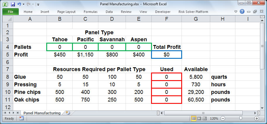
Notice that the profit for each pallet of panels ($450, $1,150, $800 and $400) was entered in cells B5, C5, D5 and E5, respectively. This allows us to compute the objective in cell F5 as:
Formula for cell F5: =B5*B4+C5*C4+D5*D4+E5*E4
or equivalently,
Formula for cell F5: =SUMPRODUCT(B5:E5,B4:E4)
In cells B8:E11, we've entered the amount of resources needed to produce a pallet of each type of panel. For example, the value 15 in cell C9 means that 15 hours of pressing is required to produce a pallet of Pacific style panels. These numbers come directly from the formulas for the constraints shown earlier. With these values in place, we can enter a formula in cell F8 to compute the total amount of glue used for any number of pallets produced:
Formula for cell F8: =SUMPRODUCT(B8:E8,$B$4:$E$4)
We can copy this formula to cells F9:F11 to compute the total amount of pressing, pine chips, and oaks chips used. (The dollar signs in $B$4:$E$4 specify that this cell range stays constant, while the cell range B8:E8 becomes B9:E9, B10:E10, and B11:E11 in the copied formulas.) The formulas in cells F8:F11 correspond to the left hand side values of the constraints.
In cells G8:G11, we've entered the available amount of each type of resource (corresponding to the right hand side values of the constraints). This allows us to express the constraints shown earlier as:
F8:F11<=G8:G11
This is equivalent to the four constraints: F8<=G8, F9<=G9, F10<=G10, and F11<=G11. We can enter this set of constraints directly in the Solver dialogs along with the non-negativity conditions:
B4:E4 >= 0
Click on the links below to see how this model can be solved using Excel's built-in Solver (or Premium Solver) or with FrontLine Systems' flagship Risk Solver Platform product.<< Back to: Tutorial Start Next: Using Excel's Solver >
Next: Using Risk Solver Platform >