This example illustrates how to use Analytic Solver Data Science's Exponential Smoothing technique to uncover trends in a time series. On the Data Science ribbon, from the Applying Your Model tab, select Help - Examples, then select Forecasting/Data Mining Examples, and open the example data set, Airpass.xlsx. This data set contains the monthly totals of international airline passengers from 1949-1960. After the example data set opens, click a cell in the data set, then on the Data Science ribbon, from the Time Series tab, select Partition to open the Time Series Partition Data dialog.
At Time Variable, select Month, and in the Variables in the Partition Data list, select Passengers. Click OK to partition the data into Training and Validation sets. (Partitioning is optional. Smoothing techniques may be run on full, unpartitioned data sets.)
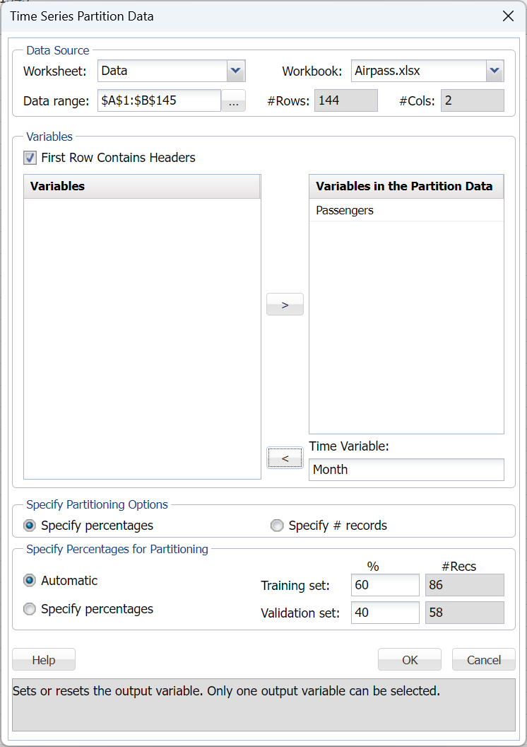
Then click OK to partition the data into training and validation sets. (Partitioning is optional. Smoothing techniques may be run on full unpartitioned datasets.) The result of the partition, TSPartition, is inserted right of the Airpass worksheet.
Click Smoothing – Exponential to open the Exponential Smoothing dialog.
Select Month as the Time Variable, unless already selected. Select Passengers as the Selected variable and also Produce Forecast on validation.
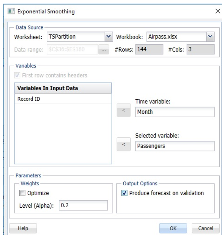
Click OK to apply the smoothing technique. Expo and Expo_Stored will be inserted right of the Data worksheet. See the “Scoring New Data” chapter for information on the Expo_Stored sheet.
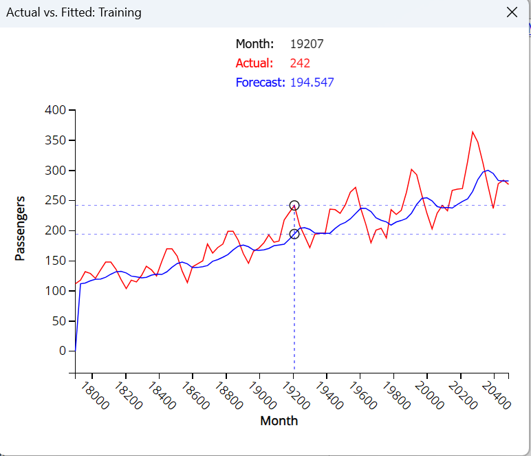
The Actual Vs Fitted: Training chart shows that the Exponential smoothing technique does not result in a good fit as the model does not effectively capture the seasonality in the dataset. As a result, the summer months where the number of airline passengers are typically high appear to be under forecasted (i.e. too low) and the forecasts for months with low passenger numbers are too high. Consequently, an exponential smoothing forecast should never be used when the dataset includes seasonality. An alternative would be to perform a regression on the model and then apply this technique to the residuals.
Note: To view these two charts in the Cloud app, click the Charts icon on the Ribbon, select Expo for Worksheet and Time Series Training Data or Time Series Validation Data for Chart.
Now let’s take a look at an example that does not include seasonality. Click Partition within the Time Series group on the Data Science ribbon to open the Time Series Partition dialog. First partition the dataset into training and validation sets using Year as the Time Variable and CA as the Variables in the partition data.
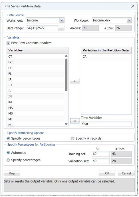
Click OK to accept the partitioning defaults and create the two sets (Training and Validation). TSPartition is inserted right of the Income worksheet. Click Smoothing – Exponential from the Data Science ribbon to open the Exponential Smoothing dialog.
Select Year for Time Variable if it has not already been selected. Select CA as the Selected Variable and Produce forecast on validation.
The smoothing parameter (Alpha) determines the magnitude of weights assigned to the observations. For example, a value close to 1 would result in the most recent observations being assigned the largest weights and the earliest observations being assigned the smallest weights. A value close to 0 would result in the earliest observations being assigned the largest weights and the latest observations being assigned the smallest weights. As a result, the value of Alpha depends on how much influence the most recent observations should have on the model.
Analytic Solver includes the Optimize feature that will choose the Alpha parameter value that results in the minimum residual mean squared error. It is recommended that this feature be used carefully as it can often lead to a model that is overfit to the training set. An overfit model rarely exhibits high predictive accuracy in the validation set.
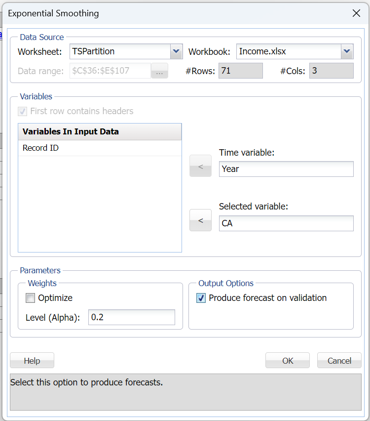
If we click OK to accept the default Alpha value of 0.2. Two output sheets, Expo and Expo_Stored, will be inserted right of the Data worksheet. For more information on the Expo_Stored worksheet, see the chapter “Scoring New Data” in the Analytic Solver Data Science User Guide.
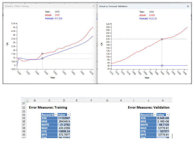
The Training and Validation Error Measures tables show a fitted model with a MSE of 258,202.3 for the Training set and a MSE of 2.16E08 for the Validation set. These are fairly large numbers and indicate that the model is not well-fit.
Note: To view these two charts in the Cloud app, click the Charts icon on the Ribbon, select Expo for Worksheet and Time Series Training Data or Time Series Validation Data for Chart.
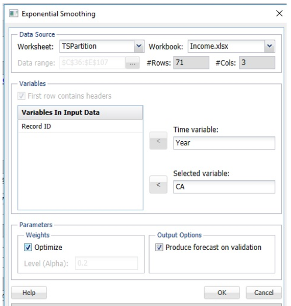
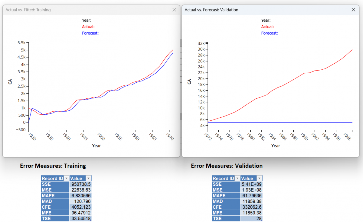
Click Smoothing – Exponential Smoothing to run the technique a second time. Again select CA as the Selected Variable and Produce forecast on validation. However, this time, select Optimize, then click OK.
Expo1 is inserted right of the Expo worksheet. Analytic Solver used an Alpha = 0.9976…
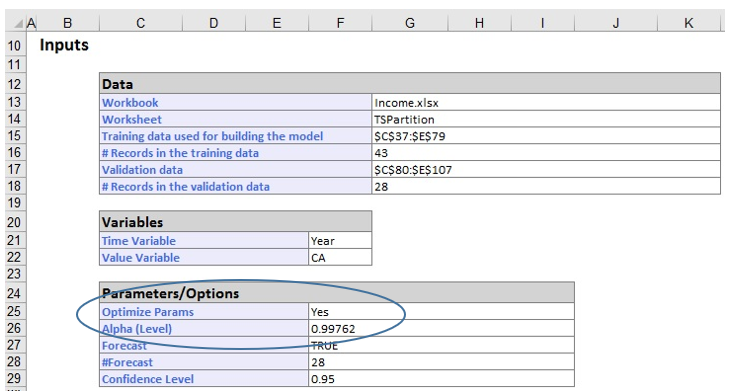
which results in a MSE of 22,110.2 for the Training Set and a MSE of 1.93E08 for the Validation Set. Although an alpha of .9976 did result in lower values, the MSE in both the training and validation sets indicates the model is still not a good fit.
Note: Click the Charts icon on the Data Science Cloud Ribbon to view the charts shown above.