This example illustrates how to use the Big Data Sample/Summarization feature by drawing a representative sample and summarizing Big Data stored across an Apache Spark compute cluster, where the Frontline Systems access server is installed. By drawing a representative sample of Big Data from all the nodes in the cluster, Excel users can train data science and text mining models directly on their desktops.
In this example, we will use the Airline data set. The data used in this example consists of flight arrival and departure information for all commercial flights within the U.S. dating from October 1987 to April 2008. This data was obtained from 29 commercial airlines and 3,376 airports, and consists of 3.2 million canceled flights, and 25 million flights at least 15 minutes late. This data set contains nearly 120 million records requiring 1.6 GB of storage space when compressed, and 12 GB of storage space when uncompressed. Data was obtained from the Research and Innovative Technology Administration (RITA), which coordinates the U.S. Department of Transportation research programs. Note that Southwest (WN), American Airlines (AA), United Airlines (UA), US Airways (US), Continental Airlines (CO), Delta Airlines (DL), Northwest Airlines (NW), and Alaska Airlines (AS) are the only airlines where data is available for all 20 years. Recall the annual revenue from the domestic airline industry is $157 billion. This public data set was obtained from here. Navigate to this website to explore details about the data set. For supplemental data including the location of each airport, plane type and meteorological data pertaining to each flight, click here.
The information contained in this large data set will help answer the following questions.
What airports are most prone to departure delays? What airports tend to have the most arrival delays?What are the times of day and days of week that are most susceptible to departure/arrival delay?
How can we understand flight patterns as they respond to well-known events (i.e., examining the data before and after September 2011)?
How many miles per year does each plane by carrier fly?
When is the best time of day, day of week, or time of year to fly to minimize delays?
How does the number of people flying between different locations change over time?
How well does weather predict plane delays?
Can you detect cascading failures as delays in one airport create delays in others? Are there critical links in the system?
How can we understand flight patterns between the pair of cities that you fly between most often, or all flights to and from a major airport like Chicago (ORD)?
How can we average arrival delay in minutes by flight or by year?
How many flights were cancelled, or were at least 15 minutes late?
How many flights were less than 50 miles?
Connecting to an Apache Spark Cluster
Analytic Solver Data Science communicates over the network with a Frontline-supplied, server-side software package that runs on one of the computers in the Spark cluster. The first step in connecting Analytic Solver Data Science to an Apache Spark cluster is to contact Frontline Systems Sales and Technical Support at 775-831-0300. When the server-side software package is installed, the proper entries for the cluster options are determined, they can be entered as shown in the example below.
For university instructors teaching business analytics to MBA and undergraduate business students -- using methods such as data science, optimization and simulation -- who would like to give their students hands-on experience with Big Data in decision making, and who do not have programming expertise or other data science preparation, Frontline Systems operates an Apache Spark cluster (in the cloud), on Amazon Web Services, pre-loaded with a set of publicly available Big Data data sets (such as the Airline dataset illustrated in this topic), and case studies using the data sets, that can be made available at a nominal cost for student use. For further information about this option, please contact Frontline Systems Academic Sales and Support at 775-831-0300 or academic@solver.com.
Storage Sources and Data Formats
Analytic Solver Data Science can process data from Hadoop Distributed File System (HDFS), local file systems that are visible to Spark cluster, and Amazon S3. Performance is best with HDFS, and it is recommended that you load data from a local file system or Amazon S3 into HDFS. If the local file system is used, the data must be accessible at the same path on all Spark workers, either via a network path, or by copying to the same worker location.
At present, Analytic Solver Data Science can process data in Apache Parquet and CSV (delimited text) formats. Performance is far better with Parquet, which stores data in a compressed, columnar representation. It is highly recommended that you convert CSV data to Parquet before you seek to sample or summarize the data.
Sampling from a Large Data Set
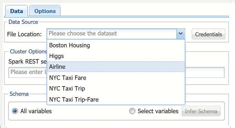
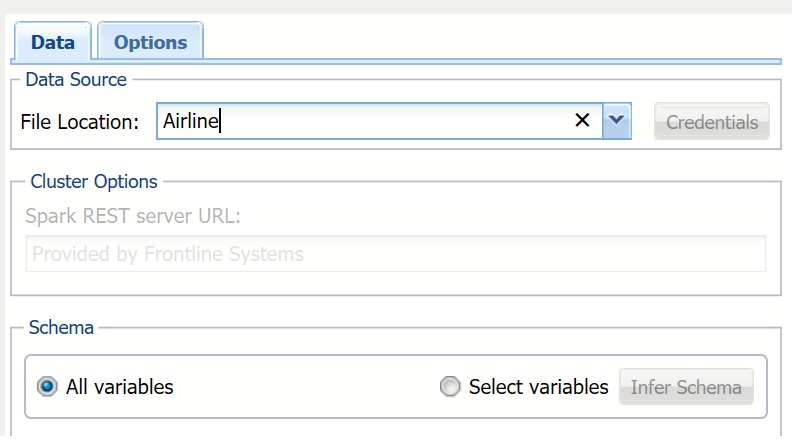
On the Analytic Solver Data Science ribbon, select Get Data - Big Data - Sample to open the Sample Big Data dialog. At File Location, enter the location of the file and the URL for the Spark Server for Spark REST server URL. This example uses the Airline data set installed on a Frontline-operated Apache Spark cluster. If your data set is located on Amazon S3, click Credentials to enter your Access Key and Secret Key.
Keep All variables selected to include all variables in the data set sample.
To only include specific variables, choose Select variables, then click Infer Schema. All variables contained in the data set are reported under Variables. Use the >/< and >>/<< buttons to select variables to be included in the sample.
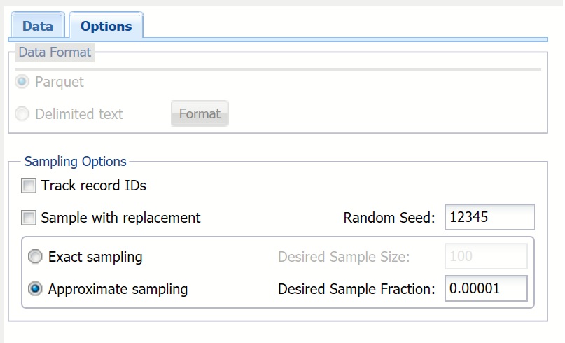
Click the Options tab.
Select Approximate sampling. When this option is selected, a sampled subset of data is returned by approximately the size of the fraction entered for Desired Sample Fraction. Approximate sampling is much faster than Exact sampling. Usually the resultant fraction is very close to the Desired Sample Fraction, making this option preferred over exact sampling. Even if the resultant sample slightly deviates from the desired size, this would be easy to correct in Excel.
Enter 0.00001 for Desired Sample Fraction. This is the expected size of the sample as a fraction of the data set's size. Since our data set contains about 120 million records, our sample will contain approximately 1,200 records. If Sampling with Replacement is selected, the value for Desired Sample Fraction is the expected number of times each record can be chosen, and must be greater than 0. If Sampling with replacement is not selected (i.e., sampling without replacement is assumed), the Desired Sample Fraction becomes the probability that each element is chosen, and Desired Sample Fraction must be between 0 and 1.
Keep Random Seed at the default of 12345. This value initializes the random number generator. Track record IDs and Sample with replacement should remain unchecked.
Please see Using Big Data for a complete description of each option included on this dialog.
Clicking Submit sends a request for sampling to the compute cluster, but does not wait for completion. The result is a worksheet containing the Job ID and basic information about the submitted job so that different submissions may be identified. This information can be used at any time to query the status of the job and generate reports based on the results of the completed job.
Clicking Run sends a request for sampling to the compute cluster and waits for the results. Once the job is completed and results are returned to the Analytic Solver Data Science client, a report is inserted into the Excel worksheet containing the sampling results.
Click Submit. The Sampling Big Data (worksheet name: BD_Sampling) report is inserted to the right of the active worksheet.
This report displays the details about the chosen data set, selected options for sampling, and the job identifier required for identifying the submission on the cluster.
On the Analytic Solver Data Science ribbon, select Get Data - Big Data - Get Results to open the Big Data: Get Results dialog. At Job identifier, click the down arrow and select the previously submitted job. Click Get Info to obtain the status of the job from the cluster.
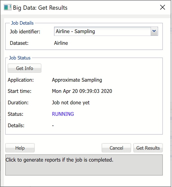
Application is the type of the submitted job. This submission corresponds to the Approximate sampling job that was submitted earlier.
Start time displays the date and time when the job was submitted. Start time will always be displayed in the user's local time.
Duration shows the elapsed time since job submission if the job is still RUNNING, and total compute time if the job is FINISHED.
Status is the current state of the job: FINISHED, FAILED, ERRORED, or RUNNING. FINISHED indicates that the job is completed and results are available for retrieval. FAILED or ERRORED indicates that the job is not completed due to an internal cluster failure. When this occurs, Details will contain a message indicating the reason.
If Status is FINISHED, click Get Results to obtain the results from the cluster and populate the report as shown below. Note that it is not required to click Get Info before Get Results. If Get Results is clicked, the status of the job is checked, and if the status is FINISHED, the results are pulled from the cluster and the report is created. Otherwise, Status is updated with the appropriate message to reflect the status: FAILED, ERRORED, or RUNNING.
Click Get Results. The worksheet BD_Sampling1 is inserted to the right of the active worksheet.
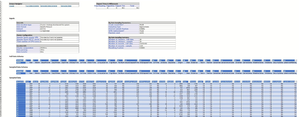
The Inputs section displays the information about the data set, cluster configuration, details on the running time, the options chosen during setup, and a summary of the data including the size and dimensionality of the full and sampled data sets. Since Approximate sampling was selected, the resulting fraction is expected to be slightly different from the desired fraction. In our example, the resulting fraction, approximately 0.00001014 (1,184/116,701,402), is very close to the requested fraction (0.00001)). Recall Approximate sampling was selected and Desired Sample Fraction was entered on the Options tab during setup.
Scroll down to see the full and sampled data schemas. Since we chose to include all variables in the sample, the set of columns in the full and sampled data sets is the same.
The Data sample includes 1,184 records, as indicated by the Number of records - sample field under Sampled Data Summary.
Now that the representative data sample has been drawn and is available in the Excel worksheet, all of the methods and features included in Analytic Solver Data Science are available. We could choose to explore the sampled data by creating visualizations using the Chart Wizard, transform the data using data transformation utilities, build classification/prediction models to forecast arrival and departure times, predict airport delays, estimate total flight times and perform any other analytic tasks that can address numerous challenges that Big Data, and the Airline data set in particular, or present the data to scientists and analysts.
Summarizing a Large Data Set
The Big Data Summarization feature in Analytic Solver Data Science translates the cluster computing capabilities from the state of the art Big Data engine, Apache Spark, to the simple, point-and-click interface within Excel. This powerful and intuitive tool is useful for rapid extraction of key metrics contained in data, which can be immediately used by data analysts and decision makers. The Summarization feature provides similar functionality as standard SQL engines, but for the data, volume, and complexity, which extends far beyond your desktop or laptop computer. This tool is a great assistant for composing reports, constructing informative visualizations, or building prescriptive and predictive models that can drive the directions of consequent analysis.
Next, we will illustrate how to utilize this easy-to-use yet powerful tool by summarizing the Airport data set and using the information obtained to answer the following three questions.
What carrier has the most domestic flights per year?Who are the most reliable airlines?
Who are the least reliable airlines?
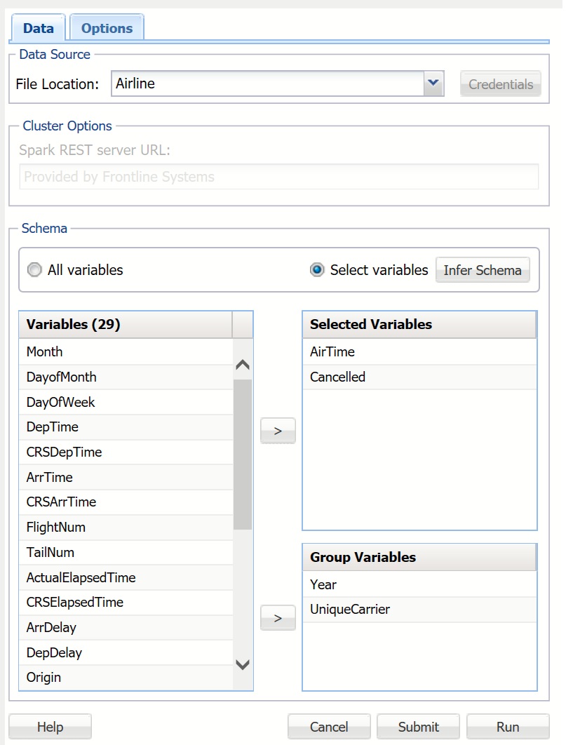
On the Analytic Solver Data Science ribbon, select Get Data - Big Data - Summarize to open the Summarize Big Data dialog. This time we will select a subset of variables for summarization along with grouping variables. After entering the File Location, Spark REST server URL, and file Credentials, select Select variables, and click Infer Schema. Transfer ArrTime and Cancelled to the Selected Variables list, and Year and UniqueCarrier to the Group Variables list. Group Variables are variables from the data set that are treated as key variables for aggregation. In this example, the variables will be grouped so that all records with the same Year and UniqueCarrier are included in the same group, and all aggregate functions for each group will be calculated.
Note: If All variables is selected, the result is a simple aggregation of all variables across the entire data set, which can be used to quickly obtain overall statistics.
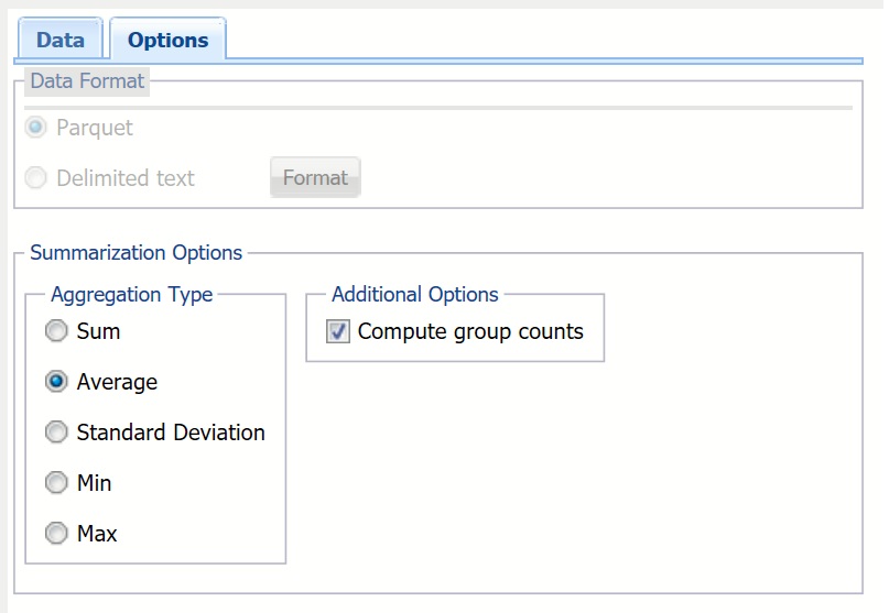
Click the Options tab to display the Summarize Big Data - Options dialog. Under Aggregation Type, select Average, and under Additional Options, select Compute group counts.
Aggregation Type provides five statistics that can be inferred from data: Sum, Average, Standard Deviation, Minimum and Maximum.
Compute group counts is enabled when 1 or more Group Variables is selected from the Summarize Big Data - Data dialog. When this option is selected, the number of records belonging to each group is computed and reported.
Click Run to send a request for a summarization job to the cluster and wait for the results. Once the job is completed, the worksheet BD_Summarization will be inserted into the current workbook and also into the Analytic Solver Data Science task pane under Transformations -- Summarize Big Data. .
In the worksheet, the Inputs section recaps the data set details, the cluster configuration, the time taken to complete the job, the options selected during setup, and the number of columns and records in both the full data set and the summarized data. Full Data Schema displays all variables in the data set, while Summarized Data Schema displays only the variables that were selected during setup.
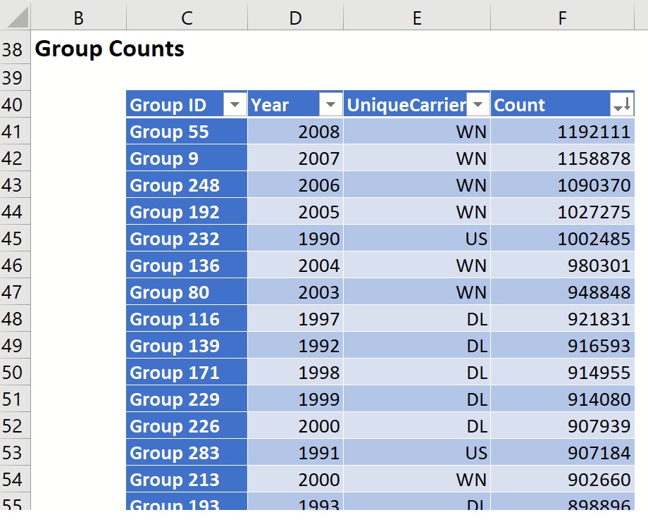
Scroll down to Group Counts to examine the number of records belonging to each Year and UniqueCarrier. In this example, there were 405,598 US Airways flights in 2003, and 684,961 Southwest flights in 1995.
Click the down arrow next to COUNT and select Sort Largest to Smallest. Once the table is sorted on the COUNT column, we can view the answer to the first question, "What carrier has the most domestic flights by year?" We see that Southwest (WN) holds the largest market share in domestic flights for years 2005-2008.

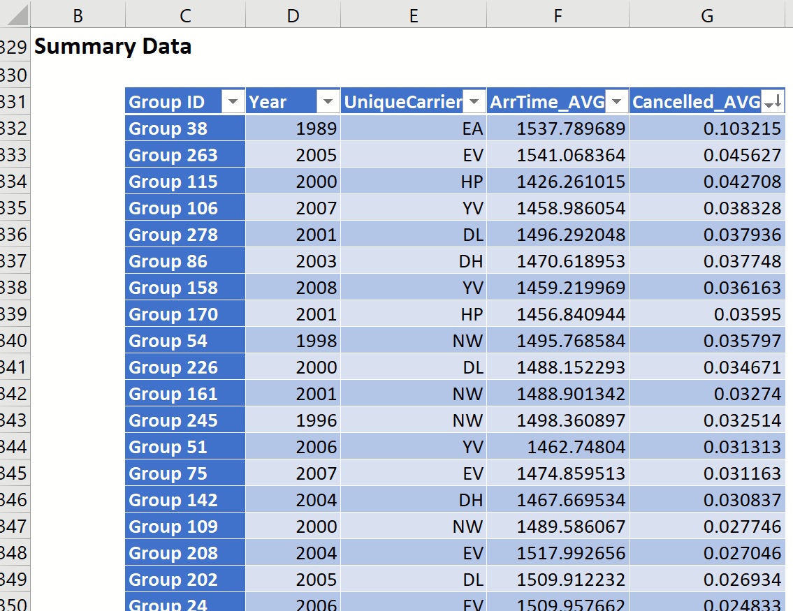
Scroll down to Summary Data to find evidence (that can be further verified) of the most and least reliable airlines. Click the down arrow next to Cancelled_AVG and sort from Largest to Smallest. The airline with the largest average percentage of canceled flights is Eastern Airlines (EA) with a little over 10% of their flights canceled on average in 1989. ExpressJet Airlines (EV) and America West (HP) round out the top three spots with 4.5% and 4.3%, respectively.
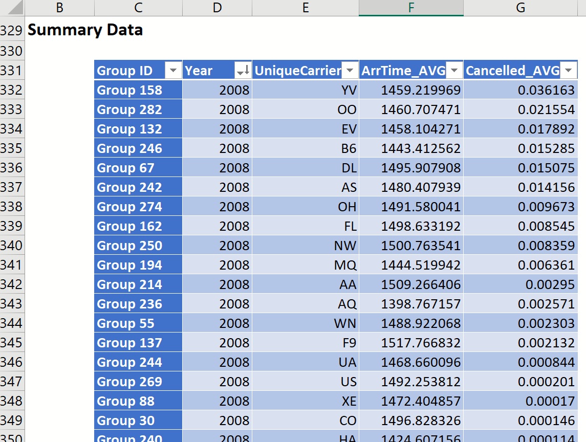
Click the down arrow next to Year and sort from Largest to Smallest. Now we see that Mesa Airlines held the largest cancellation percentage in 2008 (.036%). The second least reliable airline in 2008 goes to SkyWest Airlines (OO), with an average cancellation percentage of 2.2%, and the third least reliable airline in 2008 is awarded to ExpressJet Airlines, (EV) with an on average cancellation percentage of 1.8%.
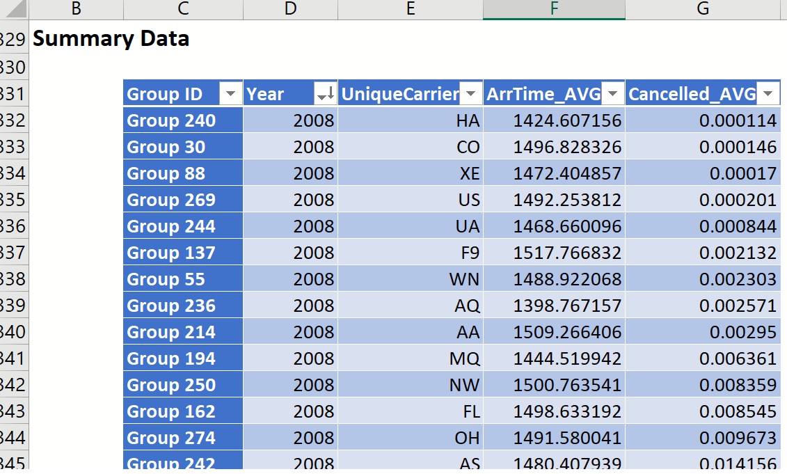
Again, click the down arrow next to Cancelled_AVG, and sort from Smallest to Largest. Then sort by Year from Largest to Smallest. The table is updated to display the airlines with the smallest on average flight cancellation percentage in 2008: 1st place - Hawaiian Airlines, 2nd place - Continental Airlines, and 3rd place - ExpressJet Airlines (1).
Using the same steps illustrated here, we could answer the following questions.
What are the yearly flight volumes per carrier?Which times of day and days of week are most susceptible to departure/arrival delays?
How many miles per year does each plane carrier fly?
Conclusion
The ability to sample and summarize large data sets is one that will become more important as technology progresses and more data is captured. Analytic Solver Data Science's Big Data feature allows users to import these large data sets into Excel allowing business analysts and data scientists the power to build predictive and prescriptive analytic models in their spreadsheets, without the need for complex programming skills.