Risk analysis is the systematic study of uncertainties and risks while Monte Carlo simulation is a powerful quantitative tool often used in risk analysis.

Uncertainty and risk are issues that virtually every business analyst must deal with, sooner or later. The consequences of not properly estimating and dealing with risk can be devastating. The 2008-2009 financial meltdown – with its many bankruptcies, homes lost to foreclosure, and stock market losses – began with inadequate estimation of risk in bonds that were backed by subprime mortgages. But in every year, there are many less-publicized instances where unexpected (or unplanned for) risks bring an end to business ventures and individual careers.
There’s a positive side to uncertainty and risk, as well: Almost every business venture involves some degree of risk-taking. Properly estimating, and planning for the upside is just as important as doing so for the downside. Risk analysis is the systematic study of uncertainties and risks we encounter in business, engineering, public policy, and many other areas. Monte Carlo simulation is a powerful quantitative tool often used in risk analysis.
Are Uncertainty and Risk Different?
Uncertainty is an intrinsic feature of some parts of nature – it is the same for all observers. But risk is specific to a person or company – it is not the same for all observers. The possibility of rain tomorrow is uncertain for everyone; but the risk of getting wet is specific to me if (a) I intend to go outdoors and (b) I view getting wet as undesirable. The possibility that stock A will decline in price tomorrow is an uncertainty for both you and me; but if you own the stock long and I do not, it is a risk only for you. If I have sold the stock short, a decline in price is a desirable outcome for me.
Many, but not all, risks involve choices. By taking some action, we may deliberately expose ourselves to risk – normally because we expect a gain that more than compensates us for bearing the risk. If you and I come to a bridge across a canyon that we want to cross, and we notice signs of weakness in its structure, there is uncertainty about whether the bridge can hold our weight, independent of our actions. If I choose to walk across the bridge to reach the other side, and you choose to stay where you are, I will bear the risk that the bridge will not hold my weight, but you will not. Most business and investment decisions are choices that involve “taking a calculated risk” – and risk analysis can give us better ways to make the calculation.
How to Deal with Risk
If the stakes are high enough, we can and should deal with risk explicitly, with the aid of a quantitative model. As humans, we have heuristics or “rules of thumb” for dealing with risk, but these don’t serve us very well in many business and public policy situations. In fact, much research shows that we have cognitive biases, such as over-weighting the most recent adverse event and projecting current good or bad outcomes too far into the future, that work against our desire to make the best decisions. Quantitative risk analysis can help us escape these biases and make better decisions.
It helps to recognize up front that when uncertainty is a large factor, the best decision does not always lead to the best outcome. The “luck of the draw” may still go against us. Risk analysis can help us analyze, document, and communicate to senior decision-makers and stakeholders the extent of uncertainty, the limits of our knowledge, and the reasons for taking a course of action.
What-If Models
The advent of spreadsheets made it easy for business analysts to “play what-if:” Starting with a quantitative model of a business situation in Excel or Google Sheets, it’s easy to change a number in an input cell or parameter, and see the effects ripple through the calculations of outcomes. If you’re reading this magazine, you’ve almost certainly done “what-if analysis” to explore various alternatives, perhaps including a “best case,” “worst case,” and “expected case.”
But trouble arises when the actual outcome is substantially worse than our “worst case” estimate – and it isn’t so great when the outcome is far better than our “best case” estimate, either. This often happens when there are many input parameters: Our “what-if analysis” exercises only a few values for each, and we never manage to exercise all the possible combinations of values for all the parameters. It doesn’t help that our brains aren’t very good at estimating statistical quantities, so we tend to rely on shortcuts that can turn out quite wrong.
Simulation Software: The Next Step
Simulation software, properly used, is a relatively easy way to overcome the drawbacks of conventional what-if analysis. We use the computer to do two things that we aren’t very good at doing ourselves:
Instead of a few what-if scenarios done by hand, the software runs thousands or tens of thousands of what-if scenarios, and collects and summarizes the results (using statistics and charts).
Instead of arbitrarily choosing input values by hand, the software makes sure that all the combinations of input parameters are tested, and values for each parameter cover the full range.
This sounds simple, but it’s very effective. There’s just one problem: If there are more than a few input parameters, and the values of those parameters cover a wide range, the number of what-if scenarios needed to be comprehensive is too great, even for today’s fast computers. For example, if we have just 10 suppliers, and the quantities of parts they supply have just 10 different values, there are 1010 or 10 billion possible scenarios. Even an automated run of 1,000 or 10,000 scenarios doesn’t come close. What can we do?
The Monte Carlo method was invented by scientists working on the atomic bomb in the 1940s. It was named for the city in Monaco famed for its casinos and games of chance. They were trying to model the behavior of a complex process (neutron diffusion). They had access to one of the earliest computers – MANIAC – but their models involved so many inputs or “dimensions” that running all the scenarios was prohibitively slow. However, they realized that if they randomly chose representative values for each of the inputs, ran the scenario, saved the results, and repeated this process, then statistically summarized all their results – the statistics from a limited number of runs would quite rapidly “converge” to the true values they would get by actually running all the possible scenarios. Solving this problem was a major “win” for the United States, and accelerated the end of World War II.
Since that time, Monte Carlo methods have been applied to an incredibly diverse range of problems in science, engineering, and finance — and business applications in virtually every industry. Monte Carlo simulation is a natural match for what-if analysis in a spreadsheet.
Randomly Choosing Representative Values
Now for the hard part (not really that hard): How do we randomly choose representative values, using a computer? This is the heart of the Monte Carlo method, and it’s where we need some probability and statistics, and knowledge of the business situation or process that we’re trying to model.
Choosing randomly is the easier part: In the external world, if there were only two possible values, we might use a coin toss, or if there were many, we might spin a roulette wheel. The analog in software is a (pseudo) random number generator or RNG – like the RAND() function in Excel. This is just an algorithm that returns an “unpredictable” value every time it is called, always falling in a range (between 0 and 1 for RAND()). The values we get from a (pseudo) random number generator are effectively “random” for our purposes, but they aren’t truly unpredictable – after all, they are generated by an algorithm. The RNG’s key property is that, over millions of function calls, the values it returns are “equidistributed” over the range specified.
To ensure that the values randomly chosen are representative of the actual input parameter, we need some knowledge of the behavior of the process underlying that parameter. Here are three histogram charts of the possible values of an input parameter. The first two are probably familiar.
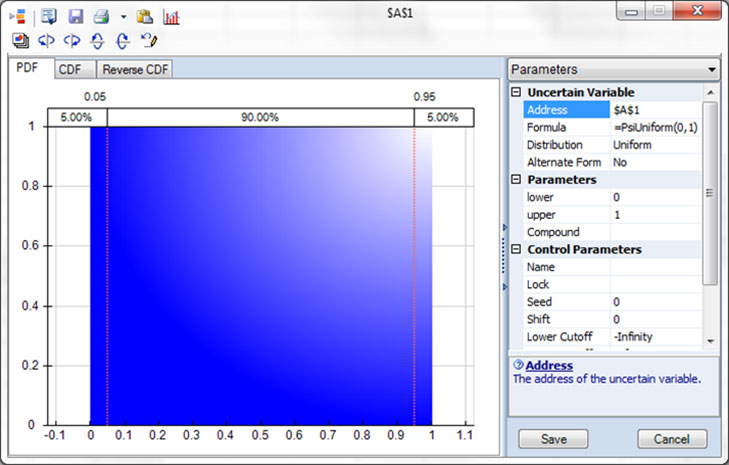
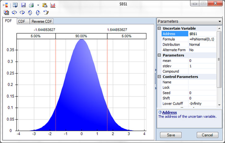
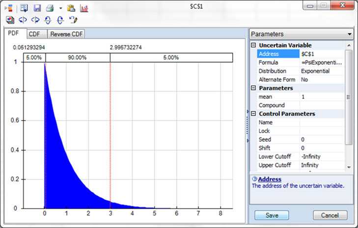
Three histogram charts of the possible values of an input parameter.
On the top is a Uniform probability distribution, where all the values between 0 and 1 are equally likely to occur. This is the distribution of values returned by the RAND() function.
In the middle is a Normal probability distribution, the most common distribution found in nature, business and the economy. Note that, unlike the Uniform distribution, the Normal distribution is unbounded – there is a small chance of very large or very small/negative values.
On the bottom is an Exponential probability distribution, which is commonly used to model failure rates of equipment or components over time. It reflects the fact that most failures occur early. Note that it has a lower bound of 0, but no strict upper bound.
Our task as business analysts is to choose a probability distribution that fits the actual behavior of the process underlying our input parameter. Most distributions have their own input parameters you can use to closely fit the values in the distribution to the values of the process. Software such as @RISK from Palisade, ModelRisk from Vose Software, and Analytic Solver Simulation from Frontline Systems (sponsors of this magazine) offers you many – 50 or more – options for probability distributions.
What Happens in a Monte Carlo Simulation
Given a random number generator and appropriate probability distributions for the uncertain input parameters, what happens when you run a Monte Carlo simulation is pretty simple: Under software control, the computer does 1,000 or 10,000 “what-if” scenario calculations – one such calculation is called a Monte Carlo “trial.” On each trial, the software uses the RNG to randomly choose a “sample” value for each input parameter, respecting the relative frequencies of its probability distribution. For example, for a Normal distribution, values near the peak of the curve will be sampled more frequently. If you’ve specified correlations, it modifies these values to respect the correlations. Then the model is calculated, and values for outputs you’ve specified are saved. It’s as simple as that!
At the end of the simulation run, you have results from 1,000 or 10,000 “what-if” scenarios. You can step through them one at a time, and inspect the results (on the spreadsheet, if you’re using one), but it’s generally easier to look at statistics and charts to analyze all the results at once. For example, here’s a histogram of one calculated result, the Net Present Value of future cash flows from a project that involves developing and marketing a new product. The chart shows a wide range of outcomes, with an average (mean) outcome of $117 million. But the full range of outcomes (in the Statistics on the right) is from negative $77.5 million to positive $295 million! And from the percentiles, we see a 5 percent chance of a negative NPV of $7.3 million or more, and a 5 percent chance of a positive NPV of $224 million or more.
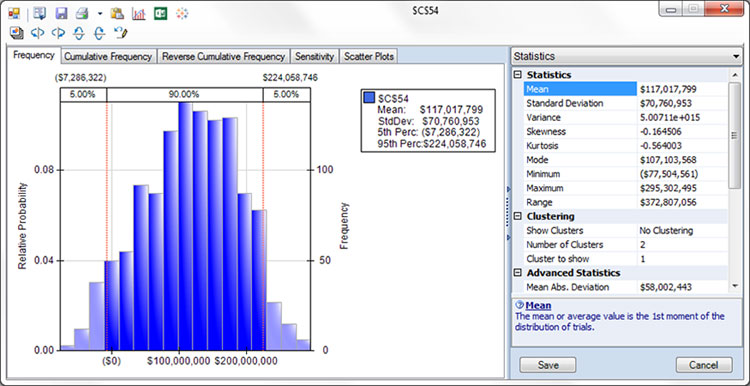
Histogram: Net Present Value of future cash flows from a project.
Another view, below, from this same chart shows us how sensitive the outcome is to certain input parameters, using “moment correlation,” one of three available presentations. $C$31 is customer demand in Year 1, $C$32 is customer demand in Year 2, and $C$35 is marketing and sales cost in Year 1 (treated as uncertain in this model). This is often called a Tornado chart, because it ranks the input parameters by their impact on the outcome, and displays them in ranked order. On the right, we are displaying Percentiles instead of summary Statistics.
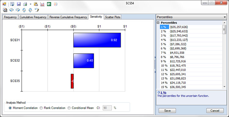
This chart shows how sensitive the outcome is to certain input parameters.
How did we construct this model? We started from a standard “what-if” model, then replaced the constant values in three input cells with “generator functions” for probability distributions. We also selected the output cell for Net Present Value, as an outcome we wanted to see from the simulation. We can pretty much always go from a what-if model to a Monte Carlo simulation model in a similar way. A chart, page 21, shows our chosen distribution – a “truncated” Normal distribution, which excludes certain extreme values – for customer demand in Year 2.
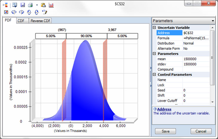
A truncated Normal distribution for customer demand in Year 2.
Steps to Build a Monte Carlo Simulation Model
If you have a good “what-if” model for the business situation, the steps involved in creating a Monte Carlo simulation model for that situation are straightforward:
- Identify the input parameters that you cannot predict or control. Different software may call these “inputs,” “forecasts,” or “uncertain variables” (Analytic Solver’s term). For these parameters (input cells in a spreadsheet), you will replace fixed numbers with a “generator function” based on a specific probability distribution.
- Choose a probability distribution for each of these input parameters. If you have historical data for the input parameter, you can use “distribution fitting” software (included in most products) to quickly see which distributions best fit the data, and automatically fit the distribution parameters to the data. Software makes it easy to place the generator function for this distribution into the input parameter cell.
- If appropriate, define correlations between these input parameters. Sometimes, you know that two or more uncertain input parameters are related to each other, even though they aren’t predictable. Using tools such as rank-order correlation or copulas, which modify the behavior of the generator functions in a simulation, you can take this into account.
Thinking about the first step, if you can predict the value of an input parameter, it’s really a constant in the model. But if you have a prediction that’s only an estimate in a range—or within ‘confidence intervals’—then it should be replaced with a generator function. If you can control the value, this parameter is really a decision variable that can be used later in simulation-based what-if analysis, or in simulation optimization.
Thinking about the third step: If you know the exact relationship between input parameter A and input parameter B (say that B = 2*A), you can just define a probability distribution for A, and use a formula to calculate B. Correlation methods are intended for cases where you know there is a relationship, but the exact form of that relationship is uncertain. For example, airline stocks tend to rise when oil stocks fall, because both are influenced by the price of crude oil and jet fuel – but the relationship is far from exact.
So, Why Do This?
We’ve seen that it really isn’t very difficult to go from a good what-if model to a Monte Carlo simulation model. The main effort is focusing on the real uncertainties in the business situation, and how you can accurately model them. The software does all the work to analyze thousands of what-if scenarios, and it gives you a new visual perspective on all of them at once.
We also saw at the beginning of this tutorial that uncertainty and risk are present in virtually every business situation, and indeed most life situations – and the consequence of not estimating risk properly, and taking steps to mitigate it, can mean an early career end, or even a business failure. That’s just the negative side – risk analysis can also show you that there’s more upside than you ever imagined.
With the effort so modest and the payoff so great, the answer should be obvious: Monte Carlo simulation should be a frequently-used tool in every business analyst’s toolkit.