Analytic Solver Data Science offers three powerful ensemble methods for use with Regression: bagging (bootstrap aggregating), boosting, and random trees. Analytic Solver Data Science Regression Algorithms on their own can be used to find one model that results in good predictions for the new data. We can view the statistics and confusion matrices of the current predictor to see if our model is a good fit to the data, but how would we know if there is a better predictor just waiting to be found? The answer is that we do not know if a better predictor exists. However, ensemble methods allow us to combine multiple “weak” regression models which, when taken together form a new, more accurate “strong” regression model. These methods work by creating multiple diverse regression models, by taking different samples of the original dataset, and then combining their outputs. (Outputs may be combined by several techniques for example, majority vote for classification and averaging for regression. This combination of models effectively reduces the variance in the “strong” model. The three different types of ensemble methods offered in Analytic Solver Data Science (bagging, boosting, and random trees) differ on three items: 1.The selection of training data for each predictor or “weak” model, 2.How the “weak” models are generated and 3. How the outputs are combined. In all three methods, each “weak” model is trained on the entire training dataset to become proficient in some portion of the dataset.
Bagging, or bootstrap aggregating, was one of the first ensemble algorithms ever to be written. It is a simple algorithm, yet very effective. Bagging generates several training data sets by using random sampling with replacement (bootstrap sampling), applies the regression model to each dataset, then takes the average amongst the models to calculate the predictions for the new data. The biggest advantage of bagging is the relative ease that the algorithm can be parallelized which makes it a better selection for very large datasets.
Boosting, in comparison, builds a “strong” model by successively training models to concentrate on records receiving inaccurate predicted values in previous models. Once completed, all predictors are combined by a weighted majority vote. Analytic Solver Data Science offers three different variations of boosting as implemented by the AdaBoost algorithm (one of the most popular ensemble algorithms in use today): M1 (Freund), M1 (Breiman), and SAMME (Stagewise Additive Modeling using a Multi-class Exponential).
Adaboost.M1 first assigns a weight (wb(i)) to each record or observation. This weight is originally set to 1/n and will be updated on each iteration of the algorithm. An original regression model is created using this first training set (Tb) and an error is calculated as:
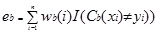 where the I() function returns 1 if true and 0 if not.
The error of the regression model in the bth iteration is used to calculate the constant αb. This constant is used to update the weight (wb(i). In AdaBoost.M1 (Freund), the constant is calculated as:
- αb= ln((1-eb)/eb)
In AdaBoost.M1 (Breiman), the constant is calculated as:
- αb= 1/2ln((1-eb)/eb)
In SAMME, the constant is calculated as:
- αb= 1/2ln((1-eb)/eb + ln(k-1) where k is the number of classes
(When the number of categories is equal to 2, SAMME behaves the same as AdaBoost Breiman.)
In any of the three implementations (Freund, Breiman, or SAMME), the new weight for the (b + 1)th iteration will be
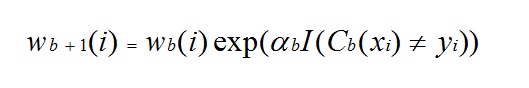
Afterwards, the weights are all readjusted to sum to 1. As a result, the weights assigned to the observations that were assigned inaccurate predicted values are increased and the weights assigned to the observations that were assigned accurate predicted values are decreased. This adjustment forces the next regression model to put more emphasis on the records that were assigned inaccurate predictions. (This α constant is also used in the final calculation which will give the regression model with the lowest error more influence.) This process repeats until b = Number of weak learners (controlled by the User). The algorithm then computes the weighted average among all weak learners and assigns that value to the record. Boosting generally yields better models than bagging, however, it does have a disadvantage as it is not parallelizable. As a result, if the number of weak learners is large, boosting would not be suitable.
Random trees, also known as random forests, is a variation of bagging. This method works by training multiple “weak” regression trees using a fixed number of randomly selected features (sqrt[number of features] for classification and number of features/3 for prediction) then takes the average value for the weak learners and assigns that value to the “strong” predictor. (This ensemble method only accepts Regression Trees as a weak learner.) Typically, in this method the number of “weak” trees generated could range from several hundred to several thousand depending on the size and difficulty of the training set. Random Trees are parallelizable since they are a variant of bagging. However, since Random Trees selects a limited amount of features in each iteration, the performance of random trees is faster than bagging.
Ensemble Methods are very powerful methods and typically result in better performance than a single tree. This feature addition in Analytic Solver Data Science (introduced in V2015) provides users with more accurate prediction models and should be considered over the single tree method.