Find Best Model Options
All options contained on the Find Best Model dialogs are described below.
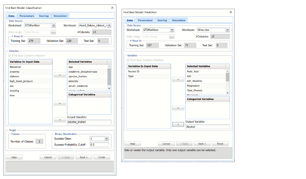
Find Best Model: Classification and Prediction, Data Tab
The Data tab is where the data source is listed, the input and output variables are selected and the Success Class and Probability are set.
Find Best Model Classification and Prediction Dialogs, Data tabs
| Workbook | Click the down arrow to select the workbook where the Find Best Model: Classification method will be applied. |
| Worksheet | Click the down arrow to select the worksheet where the Find Best Model: Classification method will be applied. |
| Data range | Select the range where the data appears on the selected worksheet. |
| #Columns |
(Read-only) The number of columns in the data range. |
| #Rows In: Training Set | (Read-only) The number of rows in the training partition. |
| #Rows In: Validation Set | (Read-only) The number of rows in the validation partition. |
| #Rows In: Test Set |
(Read-only) The number of rows in the test partition. |
| First Row Contains Headers | Select this option if the first row of the dataset contains column headings. |
| Variables in Input Data | Variables contained in the dataset. |
| Selected Variables |
Variables appearing under Selected Variables will be treated as continuous. |
| Categorical Variables | Variables appearing under Categorical Variables will be treated as categorical. |
| Output Variable |
Select the output variable, or the variable to be classified, here. |
| Classes: Number of Classes | (Read-only) The number of classes that exist in the output variable. |
| Binary Classification Success Class | This option is selected by default. Select the class to be considered a “success” or the significant class. This option is enabled when the number of classes in the output variable is equal to 2. |
| Binary Classification: Success Probability Cutoff |
Enter a value between 0 and 1 here to denote the cutoff probability for success. If the calculated probability for success for an observation is greater than or equal to this value, than a “success” (or a 1) will be predicted for that observation. If the calculated probability for success for an observation is less than this value, then a “non-success” (or a 0) will be predicted for that observation. The default value is 0.5. This option is only enabled when the # of classes is equal to 2. |
Find Best Model: Classification and Prediction, Parameters Tabs
Find Best Model Classification and Prediction Dialogs, Parameters tabs
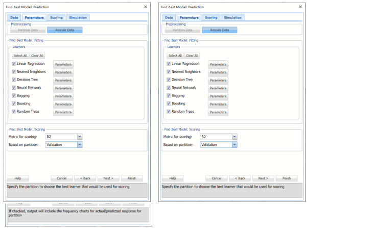
Select Find Best Model parameters here such as the learners to be applied, and their options, and the metric and partition to be used to measure the performance of each learner.
| Partition Data |
Analytic Solver Data Science includes the ability to partition a dataset from within a classification or prediction method by clicking Partition Data on the Parameters tab. Analytic Solver Data Science will partition your dataset (according to the partition options you set) immediately before running the classification method. If partitioning has already occurred on the dataset, this option will be disabled. For more information on partitioning, please see the Data Science Partitioning chapter. |
| Rescale Data | Use Rescaling to normalize one or more features in your data during the data preprocessing stage. Analytic Solver Data Science provides the following methods for feature scaling: Standardization, Normalization, Adjusted Normalization and Unit Norm. For more information on this feature, see the Rescale Continuous Data section within the Transform Continuous Data chapter that occurs earlier in this guide. |
 |
| Select All | Click to select all available learners. |
| Clear All | Click to deselect all previously selected learners. |
| Learners |
Select to run the desired Learner. Click the Parameters button to change a learner-specific option. |
| Metric for Scoring | Select the down arrow to select the metric to determine the best fit model. See the tables below for a description of each metric. |
| Based on partition | Select the down arrow to select the metric in the desired partition to determine the best fit model. |
| Logistic Regression | ||
| Fit Intercept | When this option is selected, the default setting, Analytic Solver Data Science will fit the Logistic Regression intercept. If this option is not selected, Analytic Solver Data Science will force the intercept term to 0. | |
| Iterations (Max) | Estimating the coefficients in the Logistic Regression algorithm requires an iterative non-linear maximization procedure. You can specify a maximum number of iterations to prevent the program from getting lost in very lengthy iterative loops. This value must be an integer greater than 0 or less than or equal to 100 (1< value <= 100). | |
| K-Nearest Neighbors | ||
| #Neighbors (k) | Enter a value for the parameter K in the Nearest Neighbor algorithm. | |
| Classification Tree | ||
| Tree Growth Levels, Nodes, Splits, Tree Records in Terminal Nodes | In the Tree Growth section, select Levels, Nodes, Splits, and Records in Terminal Nodes. Values entered for these options limit tree growth, i.e. if 10 is entered for Levels, the tree will be limited to 10 levels. | |
| Prune |
If a validation partition exists, this option is enabled. When this option is selected, Analytic Solver Data Science will prune the tree using the validation set. Pruning the tree using the validation set reduces the error from over-fitting the tree to the training data. Click Tree for Scoring to click the Tree type used for scoring: Fully Grown, Best Pruned, Minimum Error, User Specified or Number of Decision Nodes. |
|
| Neural Network | ||
| Architecture |
Click Add Layer to add a hidden layer. To delete a layer, click Remove Layer. Once the layer is added, enter the desired Neurons. |
|
| Hidden Layer | Nodes in the hidden layer receive input from the input layer. The output of the hidden nodes is a weighted sum of the input values. This weighted sum is computed with weights that are initially set at random values. As the network “learns”, these weights are adjusted. This weighted sum is used to compute the hidden node’s output using a transfer function. The default selection is Sigmoid. | |
| Output Layer | As in the hidden layer output calculation (explained in the above paragraph), the output layer is also computed using the same transfer function as described for Activation: Hidden Layer. The default selection is Sigmoid. | |
| Training Parameters | Click Training Parameters to open the Training Parameters dialog to specify parameters related to the training of the Neural Network algorithm. | |
| Stopping Rules |
Click Stopping Rules to open the Stopping Rules dialog. Here users can specify a comprehensive set of rules for stopping the algorithm early plus cross-validation on the training error. |
|
| Linear Discriminant | ||
| Bagging Ensemble Method | ||
| Number of Weak Learners |
|
|
| Weak Learner | Under Ensemble: Classification click the down arrow beneath Weak Leaner to select one of the six featured classifiers: Discriminant Analysis, Logistic Regression, k-NN, Naïve Bayes, Neural Networks, or Decision Trees. The command button to the right will be enabled. Click this command button to control various option settings for the weak leaner. | |
| Random Seed for Bootstrapping | Under Ensemble: Classification click the down arrow beneath Weak Leaner to select one of the six featured classifiers: Discriminant Analysis, Logistic Regression, k-NN, Naïve Bayes, Neural Networks, or Decision Trees. The command button to the right will be enabled. Click this command button to control various option settings for the weak leaner. | |
| Boosting Ensemble Method | ||
| Number of Weak Learners | See description above. | |
| Weak Learner | See description above. | |
| Adaboost Variant | 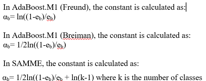 |
|
| Random Seed for Resampling | Enter an integer value to specify the seed for random resampling of the training data for each weak learner. Setting the random number seed to a nonzero value (any number of your choice is OK) ensures that the same sequence of random numbers is used each time the dataset is chosen for the classifier. The default value is “12345”. | |
| Random Trees Ensemble Method | ||
| Number of Weak Learners | See description above. | |
| Random Seed for Bootstrapping | See description above. | |
| Weak Learner | See description above. | |
| Number of Randomly Selected Features | The Random Trees ensemble method works by training multiple “weak” classification trees using a fixed number of randomly selected features then taking the mode of each class to create a “strong” classifier. The option Number of randomly selected features controls the fixed number of randomly selected features in the algorithm. The default setting is 3. | |
| Feature Selection Random Seed | If an integer value appears for Feature Selection Random seed, Analytic Solver Data Science will use this value to set the feature selection random number seed. Setting the random number seed to a nonzero value (any number of your choice is OK) ensures that the same sequence of random numbers is used each time the dataset is chosen for the classifier. The default value is “12345”. If left blank, the random number generator is initialized from the system clock, so the sequence of random numbers will be different in each calculation. If you need the results from successive runs of the algorithm to another to be strictly comparable, you should set the seed. To do this, type the desired number you want into the box. This option accepts both positive and negative integers with up to 9 digits. |
| Find Best Model Classification Scoring Statistic | Description | Find Best Model Prediction Scoring Statistic | Description | |
| R2 |  |
Accuracy | Accuracy refers to the ability of the classifier to predict a class label correctly. | |
| SSE |  |
Specificity | Specificity is defined as the proportion of negative classifications that were actually negative. | |
| MSE |  |
Sensitivity | Sensitivity is defined as the proportion of positive cases there were classified correctly as positive. | |
|
RMSE |
 |
Precision | Precision is defined as the proportion of positive results that are truly positive. | |
| MAD | 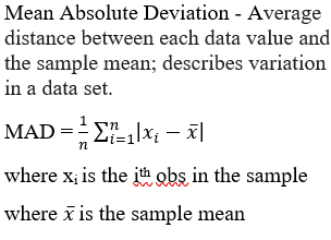 |
F1 |
Calculated as 0.743 –2 x (Precision * Sensitivity)/(Precision + Sensitivity) The F-1 Score provides a statistic to balance between Precision and Sensitivity, especially if an uneven class distribution exists. The closer the F-1 score is to 1 (the upper bound) the better the precision and recall. |
Find Best Model: Classification & Prediction Scoring tab
Find Best Model Classification and Prediction Dialogs, Scoring tab
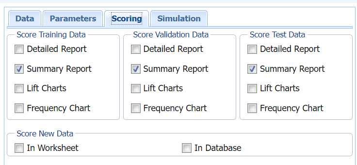
Select the type of output for the Find Best Model method and/or a scoring method (all optional).
When Frequency Chart is selected, a frequency chart will be displayed when the FBM_TrainingScore worksheet is selected. This chart will display an interactive application similar to the Analyze Data feature, explained in detail in the Analyze Data chapter that appears earlier in this guide. This chart will include frequency distributions of the actual and predicted responses individually, or side-by-side, depending on the user’s preference, as well as basic and advanced statistics for variables, percentiles, six sigma indices.
| Detailed Report | Select this option to add a Detailed Report to the output. This report shows the classification/prediction of records by row. |
| Summary Report | Select this option to add a Summary Report to the output. This report summarizes the Detailed Report. For classification models, the Summary Report contains a confusion matrix, error report and various metrics: accuracy, specificity, sensitivity, precision and F1. For regression models, the Summary Report contains five metrics: SSE, MSE, RMSE, MAD and R2. |
| Lift Charts | Select this option to add Lift charts, gain charts, and ROC curves to the output. For a description of each, see the Find Best Model chapter within the Data Science User Guide. |
| Frequency Chart |
When Frequency Chart is selected, a frequency chart will be displayed when the CFBM_TrainingScore, CFBM_ValidationScore, PFBM_TrainingScore or PFBM_ValidationScore worksheets are selected. This chart will display an interactive application similar to the Analyze Data feature, explained in detail in the Analyze Data chapter that appears earlier in this guide. This chart will include frequency distributions of the actual and predicted responses individually, or side-by-side, depending on the user’s preference, as well as basic and advanced statistics for variables, percentiles, six sigma indices. |
| In Worksheet | Select to score new data in the worksheet immediately after the Find Best Model method is complete. |
| In Database | Select to score new data within a database immediately after the Find Best Model method is complete. |
Note: See the Scoring chapter in the Data Science User Guide for more information on scoring new data.
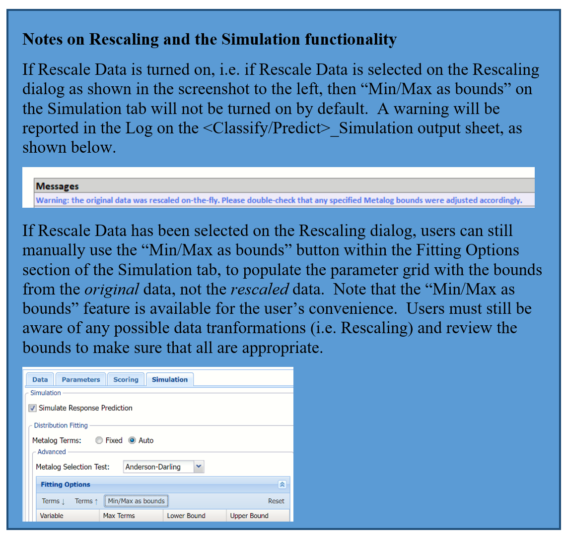
Find Best Model: Classification/Prediction Simulation tab
Find Best Model Classification and Prediction Dialogs, Simulation tab
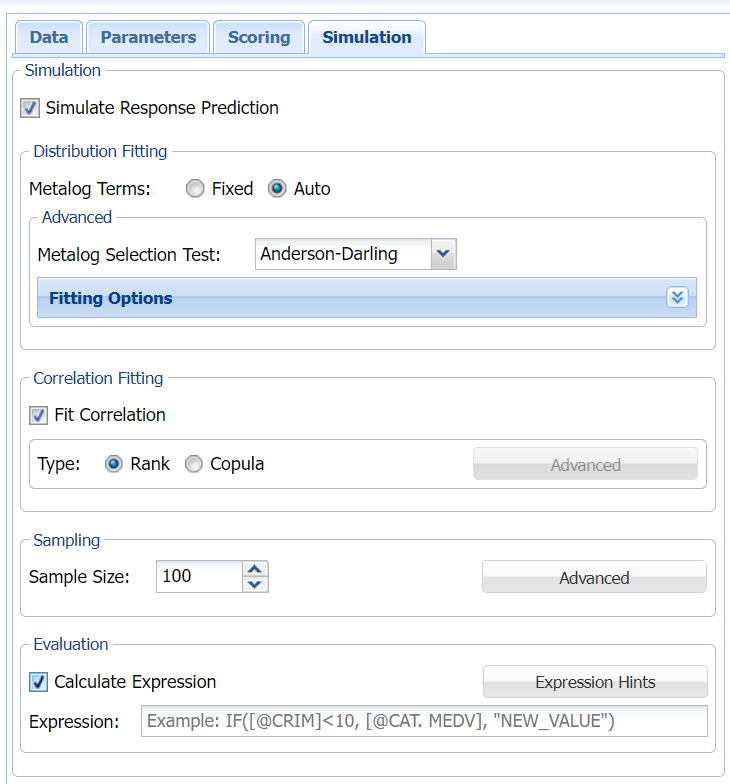
All supervised algorithms include a new Simulation tab in Analytic Solver Comprehensive and Analytic Solver Data Science. (This feature is not supported in Analytic Solver Optimization, Analytic Solver Simulation or Analytic Solver Upgrade.) This tab uses the functionality from the Generate Data feature (described earlier in this guide) to generate synthetic data based on the training partition, and uses the fitted model to produce predictions for the synthetic data. The resulting report, CFBM_Simulation (for classification) or PFBM_Simulation (for prediction) , will contain the synthetic data, the predicted values and the Excel-calculated Expression column, if present. In addition, frequency charts containing the Predicted, Training, and Expression (if present) sources or a combination of any pair may be viewed, if the charts are of the same type.
Evaluation: Select Calculate Expression to amend an Expression column onto the frequency chart displayed on the CFBM_Simulation output tab. Expression can be any valid Excel formula that references a variable and the response as [@COLUMN_NAME]. Click the Expression Hints button for more information on entering an expression.