Hierarchical Clustering Examples
Two examples are used in this section to illustrate how to use Hierarchical Clustering. The first example uses Raw Data and the second example uses a distance matrix.
Hierarchical Clustering Using Raw Data Example
The utilities.xlsx example dataset (shown below) holds corporate data on 22 US public utilities. This example will illustrate how a user could use Analytic Solver Data Science to perform a cluster analysis using hierarchical clustering.
Open this example by clicking Help – Example Models -- Forecasting/Data Science Examples – Utilities.
Each record includes 8 observations. Before Hierarchical clustering is applied, the data will be “normalized”, or “standardized”. A popular method for normalizing continuous variables is to divide each variable by its standard deviation. After the variables are standardized, the distance can be computed between clusters using the Euclidean metric.

An explanation of the variables is contained in the table below.
- X1: Fixed-charge covering ratio (income/debt)
- X2: Rate of return on capital
- X3: Cost per KW capacity in place
- X4: Anuual Load Factor
- X5: Peak KWH demand growth from 1974 to 1975
- X6: Sales (KWH use per year)
- X7: Percent Nuclear
- X8: Total fuel costs (cents per KWH)
An economist analyzing this data might first begin her analysis by building a detailed cost model of the various utilities. However, to save a considerable amount of time and effort, she could instead cluster similar types of utilities, build a detailed cost model for just one ”typical” utility in each cluster, then from there, scale up from these models to estimate results for all utilities. This example will do just that.
Click Cluster -- Hierarchical Clustering to bring up the Hierarchical Clustering dialog.
On the Data tab, Select variables x1 through x8 in the Variables in Input Data field, then click > to move the selected variables to the Selected Variables field.
Leave Data Type at Raw Data at the bottom of the dialog.
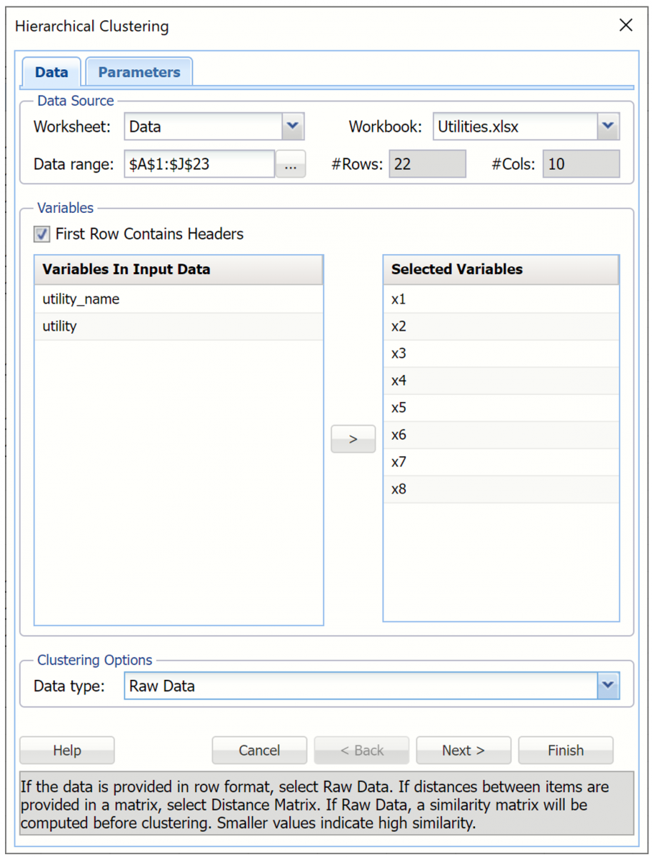
Then click Next to advance to the Hierarchical Clustering.
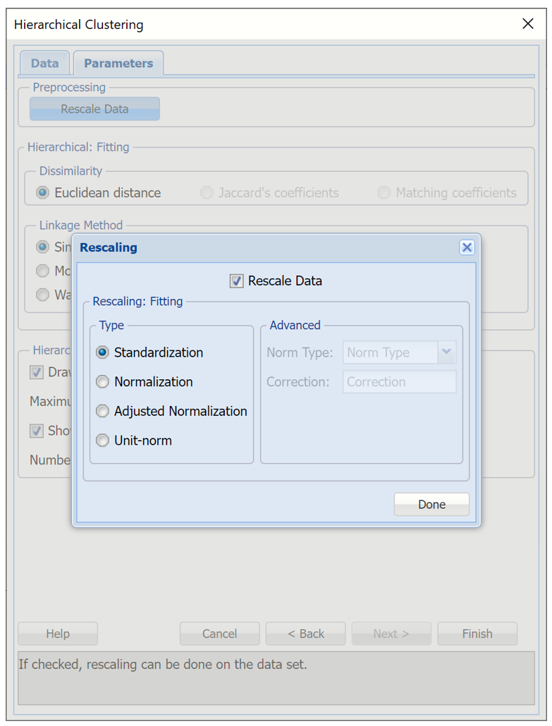
At the top of the dialog, select Rescale data. Use this dialog to normalize one or more features in your data during the data preprocessing stage. Analytic Solver Data Science provides the following methods for feature scaling: Standardization, Normalization, Adjusted Normalization and Unit Norm. For more information on this feature, see the Rescale Continuous Data section within the Transform Continuous Data chapter that occurs earlier in this guide. For this example keep the default setting of Standardization. Then click Done to close the dialog.
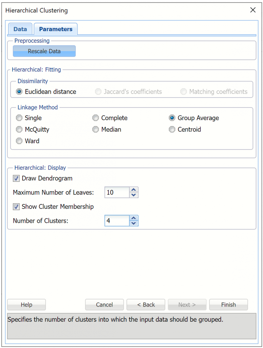
Under Dissimilarity, Euclidean distance is selected by default. The Hierarchical clustering method uses the Euclidean Distance as the similarity measure for raw numeric data.
Note: When the data is binary the remaining two options, Jaccard's coefficients and Matching coefficients are enabled.
Under Linkage Method, select Group average linkage. Recall from the Introduction to this chapter, the group average linkage method calculates the average distance of all possible distances between each record in each cluster.
For purposes of assigning cases to clusters, we must specify the number of clusters in advance. Under Hierarchical: Display, increment Number of Clusters to 4. Keep the remaining options at their defaults as shown in the screenshot below. Then click Finish.
Analytic Solver Data Science will create four clusters using the group average linkage method. The output HC_Output, HC_Clusters and HC_Dendrogram are inserted to the right of the Data worksheet.
HC_Output Worksheet
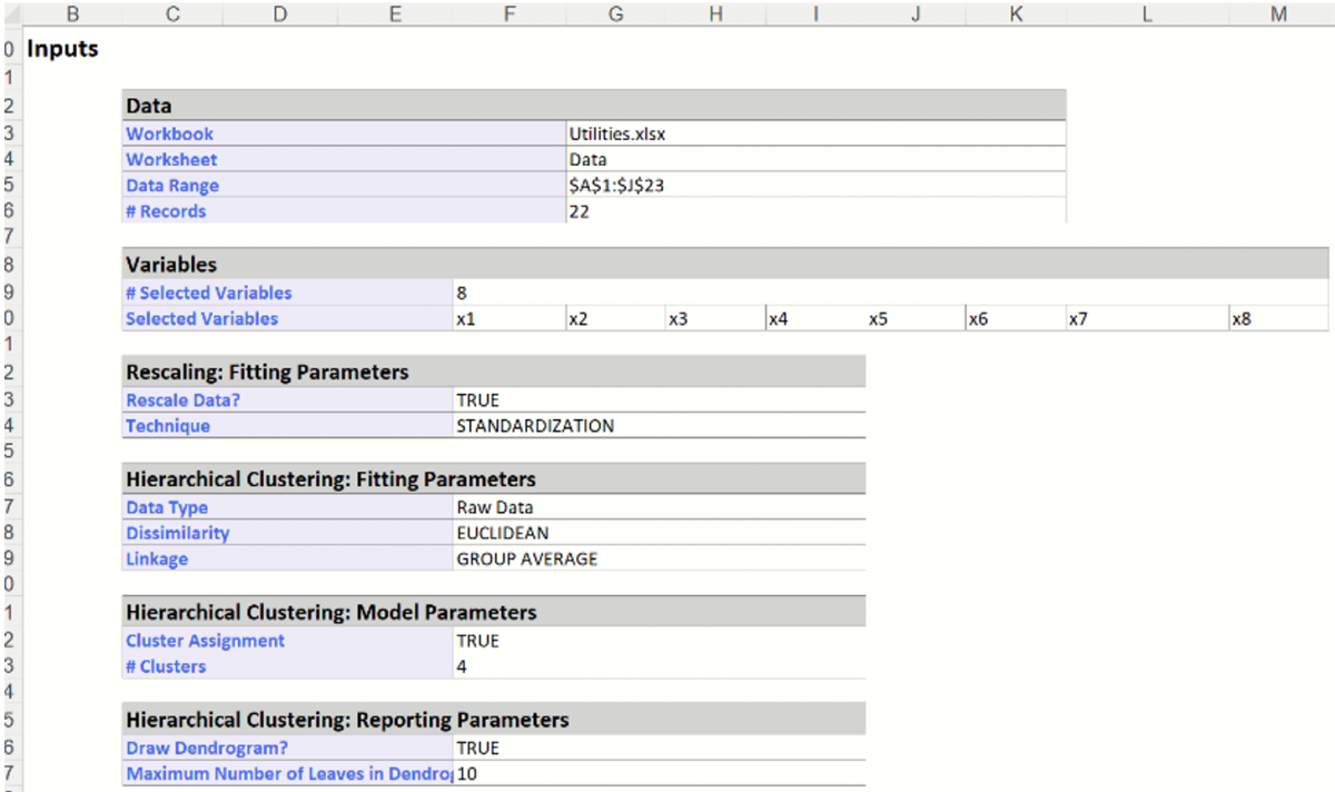
The top portion of the output simply displays the options selected on the Hierarchical Clustering dialog tabs.
Analytic Solver Data Science creates four clusters using the Group Average Linkage method. The output worksheet HC_Output is inserted immediately to the right of the Data worksheet.
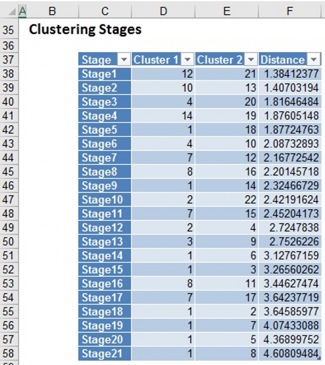
Further down the HC_Output sheet is the Clustering Stages table. This table details the history of the cluster formation. Initially, each individual case is considered its own cluster (single member in each cluster). Analytic Solver Data Science begins the method with # clusters = # cases. At stage 1, below, clusters (i.e. cases) 12 and 21 were found to be closer together than any other two clusters (i.e. cases), so they are joined together in to cluster 12. At this point there is one cluster with two cases (cases 12 and 21), and 21 additional clusters that still have just one case in each. At stage 2, clusters 10 and 13 are found to be closer together than any other two clusters, so they are joined together into cluster 10.
This process continues until there is just one cluster. At various stages of the clustering process, there are different numbers of clusters. A graph called a dendrogram illustrates these steps.
HC_Dendrogram Output
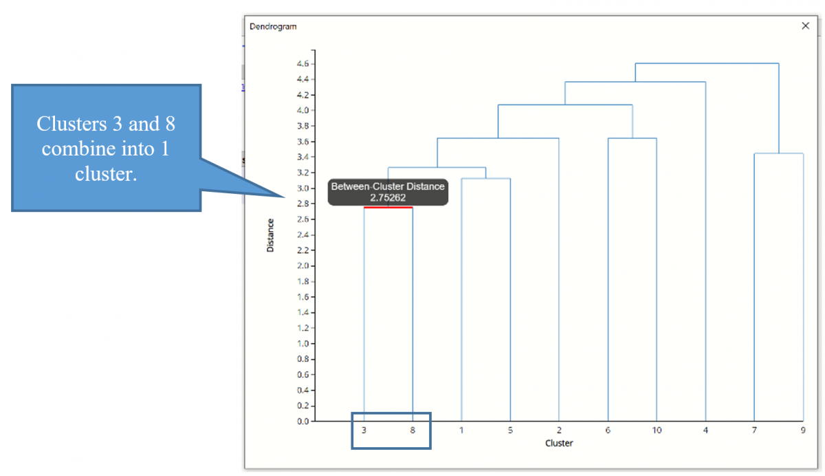
Click the HC_Dendrogram worksheet tab to view the clustering dendrogram. A dendrogram is a diagram that illustrates the hierarchical association between the clusters.
The Sub Cluster IDs are listed along the x-axis (in an order convenient for showing the cluster structure). The y-axis measures inter-cluster distance. Consider Cluster IDs 3 and 8-- they have an inter-cluster distance of 2.753. (Hover over the horizontal connecting line to see the Between-Cluster Distance.) No other cases have a smaller inter-cluster distance, so 3 and 8 are joined into one cluster, indicated by the horizontal line linking them.
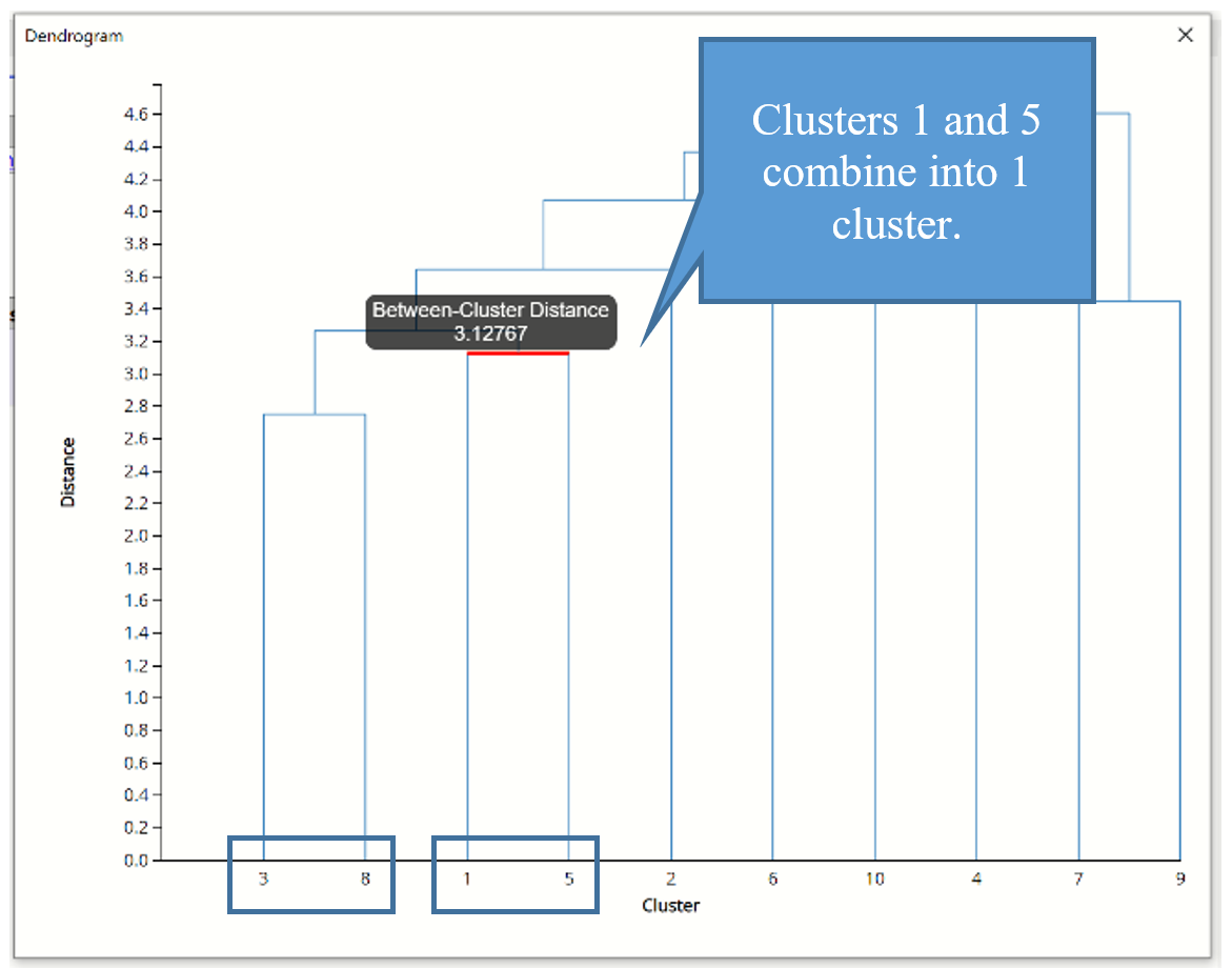
Next, we see that cases 1 and 5 have the next smallest inter-cluster distance, so they are joined into a 2nd cluster.
The next smallest inter-cluster distance is between the newly formed 3/8 and 1/5 clusters. This process repeats until all subclusters have been formed into 1 cluster.
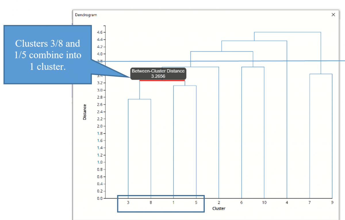
If we draw a horizontal line through the diagram at any level on the y-axis (the distance measure), the vertical cluster lines that intersect the horizontal line indicate clusters whose members are at least that close to each other. If we draw a horizontal line at distance = 3.8, for example, we see that there are 4 clusters that have an inter-cluster distance of at least 3.8. In addition, we can see that a sub ID can belong to multiple clusters, depending on where we draw the line.
Click the ‘X’ in the upper right hand corner to close the dendrogram to view the Cluster Legend. This table shows the records that are assigned to each sub-cluster.
Hierarchical Cluster Using a Distance Matrix
This next example illustrates Hierarchical Clustering when the data represents the distance between the ith and jth records. (When applied to raw data, Hierarchical clustering converts the data into the distance matrix format before proceeding with the clustering algorithm. Providing the distance measures in the data requires one less step for the Hierarchical clustering algorithm.)
Open the DistMatrix example dataset by clicking Help – Example Models – Forecasting / Data Science Examples.
Open the Hierarchical Clustering dialog by clicking Cluster – Hierarchical Clustering.
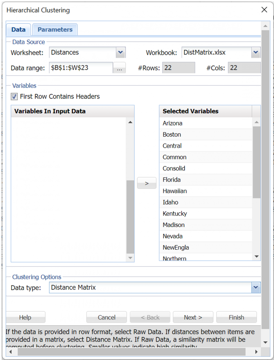
At the top of the Data tab, B1:W23 has been saved as the default for Data range.
All variables have been previously saved as Selected Variables and Distance Matrix has been selected by default.
Note: When Distance Matrix is selected, the distance matrix is validated to be a valid distance matrix (a square, symmetric matrix with 0’s on the diagonal).
Click Next.
Rescale Data is disabled since the distance matrix is used.
Keep the default, Euclidean distance, selected for Dissimilarity. (See below for explanations for Jaccard’s coefficients and Matching coefficients.)
Select Group average linkage as the Clustering Method.
Leave Draw dendrogram, Maximum Number of Leaves. Set Number of Clusters to 4.

Then click Finish.
Output worksheets are inserted to the right of the Distances tab: HC_Output, HC_Clusters, and HC_Dendrogram. The contents of HC_Output and HC_Dendrogram are described below. See above for a description of the contents of HC_Clusters.
HC_Output Worksheet
As in the example above, the top of the HC_Output worksheet is the Inputs portion, which displays the choices selected on both tabs of the Hierarchical Clustering dialog.
Scroll down to the Clustering Stages table. As discussed above, this table details the history of the cluster formation. At the beginning, each individual case was considered its own cluster, # clusters = # cases. At stage 1, below, clusters (i.e. cases) 4 and 10 were found to be closer together than any other two clusters (i.e. cases), so 4 absorbed 10. At stage 2, clusters 4 and 15 are found to be closer together than any other two clusters, so 4 absorbed 15. At this point there is one cluster with three cases (cases 4, 10 and 15), and 20 additional clusters that still have just one case in each. This process continues until there is just one cluster at stage 21.

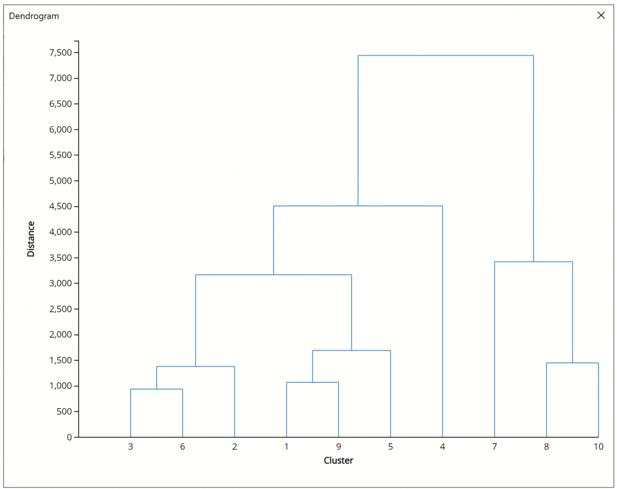
The Dendrogram output (included on HC_Dendrogram) is shown below.
Note: To view charts in the Cloud app, click the Charts icon on the Ribbon, select HC_Dendrogram for Worksheet and Dendrogram for Hierarchical Clustering for Chart.
One of the reasons why Hierarchical Clustering is so attractive to statisticians is because it’s easy to understand and the clustering process can be easily illustrated with a dendrogram. However, there are a few limitations.
- Hierarchical clustering requires computing and storing an n x n distance matrix. If using a large dataset, this requirement can be very slow and require large amounts of memory.
- Clusters created through Hierarchical clustering are not very stable. If records are eliminated, the results can be very different.
- Outliers in the data can impact the results negatively.