|
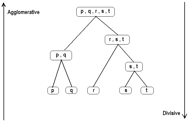
Cluster Analysis (data segmentation) has a variety of goals that relate to grouping or segmenting a collection of objects (i.e., observations, individuals, cases, or data rows) into subsets or clusters, such that those within each cluster are more closely related to one another than objects assigned to different clusters. Central to all of the goals of cluster analysis is the notion of degree of similarity (or dissimilarity) between the individual objects being clustered. There are two major methods of clustering: hierarchical clustering and k-means clustering. For information on k-means clustering, refer to the k-Means Clustering section. In hierarchical clustering, the data is not partitioned into a particular cluster in a single step. Instead, a series of partitions takes place, which may run from a single cluster containing all objects to n clusters that each contain a single object. Hierarchical Clustering is subdivided into agglomerative methods, which proceed by a series of fusions of the n objects into groups, and divisive methods, which separate n objects successively into finer groupings. Agglomerative techniques are more commonly used, and this is the method implemented in Analytic Solver Data Science. Hierarchical clustering may be represented by a two-dimensional diagram known as a dendrogram, which illustrates the fusions or divisions made at each successive stage of analysis. Following is an example of a dendrogram. |

Agglomerative methodsAn agglomerative hierarchical clustering procedure produces a series of partitions of the data, Pn, Pn-1, ....... , P1. The first Pn consists of n single object clusters, the last P1, consists of single group containing all n cases. At each particular stage, the method joins together the two clusters that are closest together (most similar). (At the first stage, this amounts to joining together the two objects that are closest together, since at the initial stage each cluster has only one object.) Differences between methods arise due to different ways of defining distance (or similarity) between clusters. The following sections describe several agglomerative techniques in detail. |
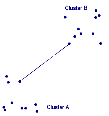
Single linkage clusteringOne of the simplest agglomerative hierarchical clustering methods is single linkage, also known as the nearest neighbor technique. The defining feature of the method is that distance between groups is defined as the distance between the closest pair of objects, where only pairs consisting of one object from each group are considered. In the single linkage method, D(r,s) is computed as At each stage of hierarchical clustering, the clusters r and s , for which D(r,s) is minimum, are merged. In this case, those two clusters are merged such that the newly formed cluster, on average, will have minimum pairwise distances between the points. |

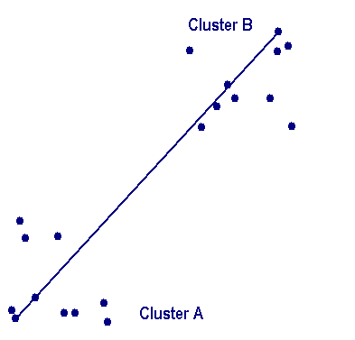
Complete linkage clusteringIn the complete linkage, also called farthest neighbor, the clustering method is the opposite of single linkage. Distance between groups is now defined as the distance between the most distant pair of objects, one from each group. In the complete linkage method, D(r,s) is computed as The distance between every possible object pair (i,j) is computed, where object i is in cluster r and object j is in cluster s and the maximum value of these distances is said to be the distance between clusters r and s. The distance between two clusters is given by the value of the longest link between the clusters. At each stage of hierarchical clustering, the clusters r and s , for which D(r,s) is maximum, are merged. |

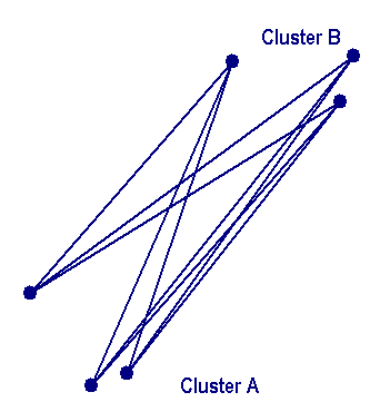
Average linkage clusteringIn Average linkage clustering, the distance between two clusters is defined as the average of distances between all pairs of objects, where each pair is made up of one object from each group. In the average linkage method, D(r,s) is computed as At each stage of hierarchical clustering, the clusters r and s , for which D(r,s) is the minimum, are merged. |

Average group linkageWith this method, groups once formed are represented by their mean values for each variable (i.e., their mean vector and inter-group distance is defined in terms of distance between two such mean vectors). In the average group linkage method, the two clusters r and s are merged such that the average pairwise distance within the newly formed cluster is minimum. Suppose we label the new cluster formed by merging clusters r and s as t. Then the distance between clusters r and s, D(r,s), is computed as |
Ward's hierarchical clustering methodWard (1963) proposed a clustering procedure seeking to form the partitions Pn, P n-1,........, P1 in a manner that minimizes the loss associated with each grouping, and to quantify that loss in a form that is readily interpretable. At each step in the analysis, the union of every possible cluster pair is considered and the two clusters whose fusion results in minimum increase in information loss are combined. Information loss is defined by Ward in terms of an error sum-of-squares criterion (ESS). The rationale behind Ward's proposal can be illustrated most simply by considering univariate data. Suppose for example, 10 objects have scores (2, 6, 5, 6, 2, 2, 2, 2, 0, 0, 0) on some particular variable. The loss of information that would result from treating the ten scores as one group with a mean of 2.5 is represented by ESS, ESS One group = (2 -2.5)2 + (6 -2.5)2 + ....... + (0 -2.5)2 = 50.5 On the other hand, if the 10 objects are classified according to their scores into four sets, {0,0,0}, {2,2,2,2}, {5}, {6,6} The ESS can be evaluated as the sum of squares of four separate error sums of squares ESS One group = ESS group1 + ESSgroup2 + ESSgroup3 + ESSgroup4 = 0.0 Thus, clustering the 10 scores into four clusters results in no loss of information. |
